Wait, it's all histograms? Simplifying our Bayesian A/B testing methodology - Part 2

Image source: Wikimedia Commons.
The Bayesian approach to A/B testing has many advantages over a Frequentist approach. However, there are some drawbacks. This post discusses these challenges and our attempts to overcome them.
A/B Testing at Auto Trader
We highly recommend first reading the companion post about our move to Bayesian A/B testing. Therein, we describe what motivated our shift and explain the base methodology.
As a quick recap: in the Bayesian approach we want to find the Posterior, \(P(Metric\|Data)\), which in plain English is the probability distribution of what we’re measuring (e.g. the click-through rate, CTR) given the data we have observed (e.g. clicks and views). We do this by combining the Likelihood \(L(Data\|Metric)\), which reflects how likely a given data-generating process will produce the values we’ve observed, with a Prior, \(P(Metric)\), which reflects our expectation of what the metric could be. A final term \(P(Data)\) normalises the above to ensure that the Posterior is a valid probability distribution, giving us Bayes rule:
\[P(Metric\|Data) = \frac{L(Data\|Metric)P(Metric)}{P(Data)}\]In the Bayesian A/B testing approach, based on the VWO Paper by Chris Stucchio, we use each variant’s Posterior to investigate the differences between the experimental groups and the control group. We can generate a metric called the Expected Loss from these Posteriors, which reflects the consequence of us choosing the wrong variant. Crucially, this is sensitive to significant mistakes. The Expected Loss can flag a slight chance of a major 10% reduction in our metric while letting a large chance of a minor 0.1% reduction slide. In practice, this means we can terminate a test containing two nearly identical variants, yielding a small Expected Loss, and decide which variant to move forward with based on other decision criteria (e.g. reducing tech debt, more consistent branding).
But what Likelihood represents my data!?
One of the key decisions someone must make when analysing an experiment is what Likelihood best represents the collected data. An incorrect choice of Likelihood can impact the accuracy of the Posterior, leading to inaccurate insights and uninformed decisions.
There is some good news. Analysts are somewhat restricted in their choice of Likelihoods to a special set of Likelihood-Prior combinations known as conjugates. These special pairs nicely combine to create a Posterior with a well-defined form. You could easily pick other non-conjugate distributions, but that leads to complicated (and finicky) sampling techniques to investigate the Posterior.
But there is bad news. Real-world data is often simply too complex to reasonably represent with a conjugate Likelihood-Prior combination. Can you define a distribution that represents the data below?
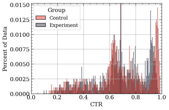
Simulated data that reflects the incredibly variable, messy reality. Vertical lines indicate the (very similar) group means.
Perhaps someone is able to find a Likelihood, or collection of combined Likelihoods, that adequately represent the above data. However, stakeholders are interested in multiple metrics, not to mention the ever-changing world (causing ever-changing distributions for any given metric). Creating bespoke models to accommodate all the changes would be a massive time-sink. Can we create a generalised solution so analysts don’t have to worry about these problems?
Everything is a histogram
While thinking about solutions, we kept looking at histograms of the data (like the one shown above). In a flash of inspiration, we realised that a histogram is actually quite similar to a Categorical distribution. The Categorical distribution represents the probability that one (and only one) of a fixed number of exclusive events occur. For instance, it could represent the probability of a customer ordering one scoop of chocolate ice cream (as opposed to vanilla, strawberry, caramel, pistachio, or coffee).
To apply this to our problem we can make a simplifying assumption. What if we simply assign any continuous (or discrete) metric we want into the appropriate bin of a Categorical? The metric in the above plot is bounded between 0 and 1, so we can simply create exclusive bins within that region and place each data point into the appropriate bin.
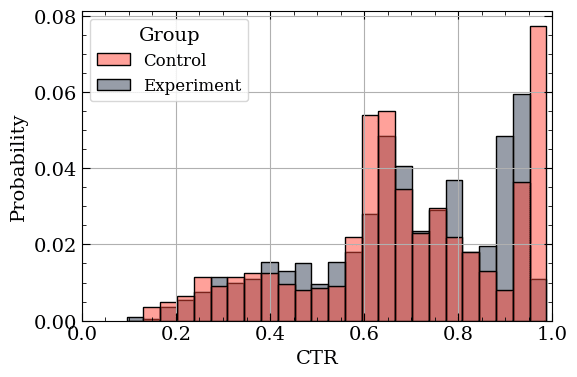
Example of Categorical distribution representations of the data using 25 bins.
The beautiful thing about the Categorical Likelihood is that it has a conjugate Prior: the Dirichlet distribution! This creates a Dirichlet Posterior that represents the chance a collection of observations will form a specific Categorical distribution. The picture below depicts the relationship between the two distributions using three colours and three bins. Each colour represents one random draw from a Dirichlet, and the Categorial distribution on the right is the shape specified by said random draw (i.e. colour).
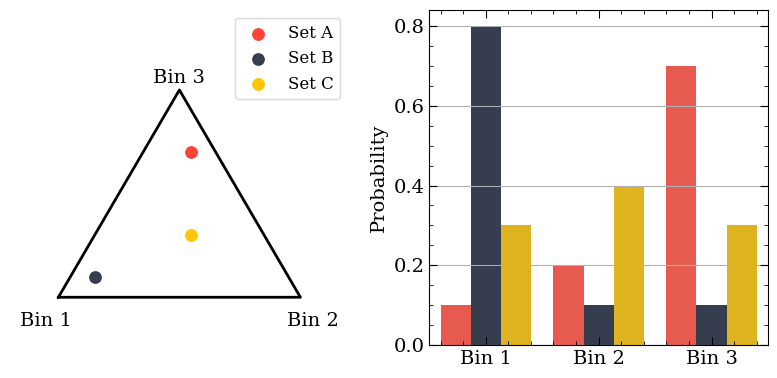
The relationship between the Dirichlet and Categorical distributions. Each colour is a random value drawn from the Dirichlet on the left; it is similarly represented as a collection of bin probabilities on the right.
Why is the Dirichlet distribution shaped like a triangle? That triangle is more formally known as a “simplex” and is quite special. Each point inside the simplex can be described with a unique set of coordinates. Think of describing your current location using latitude, longitude, and elevation. Thus, despite visually showing a single point on the left plot above, it actually corresponds to three values: the probability of going into a specific bin in the Categorical distribution on the right plot. Normally, we work with dozens, if not hundreds, of bins, but the underlying idea is the same as the plot above. As we acquire more data, the Dirichlet Posterior focuses in on the most-likely shapes our histogram-based estimation of the data can take.
But what do I do with it?
Now that we’ve represented the data using a Dirichlet-Categorical model, what do we do with it? We sample from the Dirichlet Posterior (much like we would sample from any Posterior), giving us a set of probabilities per bin. Then, we can compute the average overall value by taking the sum of the probability of being in a given bin multiplied by the “central” value of said bin.
What is the “central” value of the bin? Do you simply take the mid-point of the bin edges or the mean or median of the observations within that bin? As the number of bins increases this becomes less of a problem, but we opt for the median value of observations within the bin. This is particularly useful for bins at the extreme of the distribution.
We can repeat this sample-then-average procedure many times for the various experimental variants, creating a distribution of population averages for our metric. We can then compare these population average distributions to get our Chance to Beat and Expected Loss. Eagle-eyed readers may realise that this corresponds to the population average of the metric, not the metric as it applies to a given visitor to Auto Trader. Ongoing work seeks to use this Dirichlet-Categorical framework to represent the individual, not just the population.
But how many bins should I have?
A consequence of this binning approach is that we must explicitly define both the range of values we’ll consider and the number of bins to use. The range of values is almost always pre-decided since we remove extreme values, such as bot activity, from the data. But how many bins is sensible? To answer this, we ran many simulations using a variety of distributions with known means and variances. For each distribution type, we analysed how well the Dirichlet-Categorical approach with varying bin sizes approximated the known true values. One example is shown below.
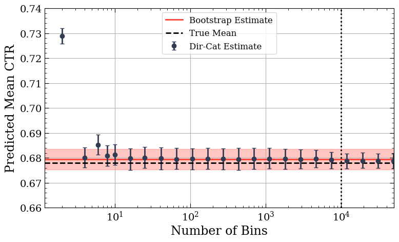
The change in the reported CTR mean and uncertainty as the number of bins increases.
In the plot above, the red horizontal shaded area and line show the bootstrapped 95% certainty range for the mean CTR. The blue dots show the mean and 95% certainty range for a Dirichlet with a given number of bins. The dashed vertical line shows the number of samples in the simulated dataset, and the horizontal dashed line shows the true expected value for the simulated dataset.
We found that aside from a near-trivial number of bins (<10), the Dirichlet-Categorical approach was remarkably stable (having clearly converged past 100 bins), producing the expected values for the various distributions we tested. The points show the mean of the values sampled from the posterior, and the error bar covers 95% of the sampled values. We see that as the number of bins approaches the number of data points, the uncertainty estimate begins to shrink below the range obtained from bootstrapping, which we will discuss in the next section.
In short, the number of bins doesn’t have much of an impact as long as you’re using more than 100 or so1.
Further validating the generalised procedure
The real gold standard for assessing the uncertainty around A/B tests is “bootstrapping”, which generates synthetic datasets from the already-acquired data. Briefly, we grab a couple thousand random samples (with replacement) from all the observations for a given variant. We then compute some value or metric from this synthetic sample and store it. The process is repeated thousands of times to create thousands of estimates for the metric. The bootstrapped distribution of the metric can then be used to estimate the uncertainty of the metric. This is a great point of comparison for the Dirichlet-Categorical approach.
As can be seen above, the Dirichlet-Categorical approach quickly overlaps the bootstrapped estimate, giving us confidence in our generalised approach. The obtained uncertainty ranges are also in good agreement, aside from the extreme case where we have the same order of bins as we have data points. In this regime, we see the Dirichlet-Categorical approach begin to underestimate the uncertainty while remaining unbiased. While this behaviour is not ideal, it occurs in the plot’s ‘for science’ range. In any practical scenario, the number of bins would be far less than the number of data points (and the dataset so small that bootstrapping would be the recommended approach). In addition, both the bootstrapped interval and the Dirichlet-Categorical approach overlap with the actual expected value of the metric (which we know because it’s a simulated dataset).
Conclusion
One of the main stumbling blocks with the roll-out of Bayesian A/B testing was the confusion over the choice of Likelihood, especially when there wasn’t a good option that matched the data. Our general approach of modelling everything as a Categorical removes the need for an analyst to pick a Likelihood. The data simply needs to be binned into a good number of buckets and then fed into our automated in-house A/B testing package. We recognise that binning feels like a somewhat controversial choice, but we are confident that it delivers accurate results. We are further testing various methods of distribution approximation and bin selection and will present a full accounting in a white paper in the coming months. The qualitative finding is that, so long as you don’t do something silly (using way too few bins, using way too many bins, etc), it works surprisingly well. We also recommend defining bin edges using quantile-spacing of your data as opposed to linear-spacing.
The generalisable Dirichlet-Categorical approach lessens the need for bespoke metric models crafted by highly knowledgeable Bayesian statisticians using a plethora of Likelihoods. Instead, we can get an approximate answer using a simple choice of bins. Since this binned approximation is often more similar to the oddly shaped data distribution, we’ve found that we can be more confident in our measured metric and its uncertainty.
[1] We appreciate the above is rather hand-wavy; we plan on producing a far more detailed paper in the future for those (rightfully!) wanting more robust evidence. ↩
Enjoyed that? Read some other posts.
Related Posts
14 Aug 2024—Tom Armitage & Dustin Hayden
Image source: Wikimedia Commons.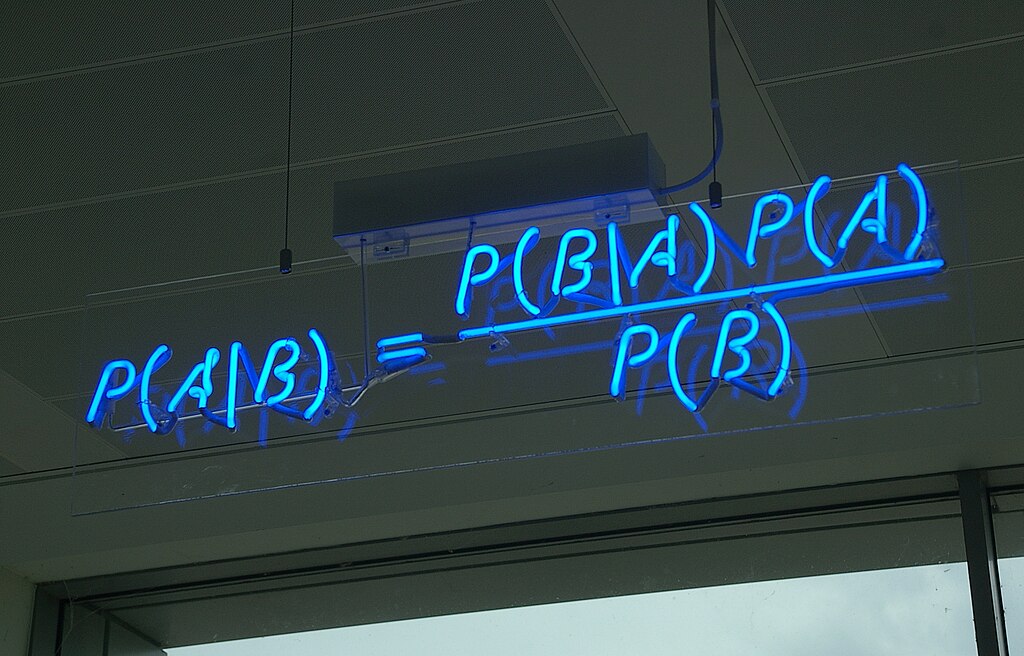
Websites are constantly changing. Here at Auto Trader, we use A/B testing to monitor the impact these changes have on the user’s experience. Fundamentally, we need to gather sufficient evidence to make a decision...
04 Jul 2024—Mahmoud Oshagh
Photo by Eugenio Mazzone on Unsplash.
Have you ever stumbled upon something that just completely captivated your attention? That was precisely what happened to me when I first came across Large Language Models (LLMs). It was during...
31 May 2024—Tom Armitage & Tom Kelly
Image source: Wikimedia Commons.
There has been great advancement in recent years in the field of image classification. With pre-trained models readily available and mature libraries making the process of developing and training your own models easy, you...
05 Oct 2023—Tim Summerton-Brier, Stevie Woods, John Harrison
Photo by Tico Mendoza
Back in April, Auto Trader gave a few of us the opportunity to attend Data Council 2023 in Austin, Texas, USA. Data Council is an independently curated conference that covers many aspects of working...
17 Apr 2023—Olivia Pennington & Tom Armitage
Photo by Nik Shuliahin on Unsplash.
You’ve done the hard work in researching, developing and finally deploying your shiny new Machine Learning (ML) model, but the work is not over yet. In fact it has only just...
24 Mar 2023—Tom Armitage & Olivia Pennington
Photo by Stephen Dawson on Unsplash.
Advertising packages are the core product at Auto Trader. Depending on the package tier our customers purchase, they get to appear in...
