Image source: Wikimedia Commons.

Websites are constantly changing. Here at Auto Trader, we use A/B testing to monitor the impact these changes have on the user’s experience. Fundamentally, we need to gather sufficient evidence to make a decision and then communicate that to stakeholders. Ensuring that the results of any test are reported accurately and clearly is vital for a productive culture of experimentation. In this post, we discuss our move to a Bayesian framework and the advantages we believe it brings to the analysis and reporting of experiments.

Motivation

The Analytics Group is responsible for the quality of the A/B testing methodologies at Auto Trader. If you would like a broader overview of experimentation, please read our previous post here. This post will delve into more details related to the various testing frameworks we’ve used. It begins by highlighting the issues with the previous approach, explores a better framework for answering common questions, and finally details how we distributed the updated framework to the entire Analytics Group.

Our previous approach

We continue with the hypothetical example from our previous post about A/B testing. Namely, we create a version of the front page that prominently features electric vehicles and randomly assign some visitors to view that front page. This is our Experimental group. We are interested in which option — experimental (electric vehicles on the front page) or control (internal combustion engine vehicles on the front page) — causes a higher click-through rate (CTR) for electric vehicles throughout a visitor’s website journey. So, how do we investigate that?

The first approach is remarkably straightforward. Merely find the average CTR for each group and make decisions based on those summary values. If, for example, the average CTR for the experimental group is higher, we would conclude that being shown an electric vehicle results in users engaging more with electric vehicles.

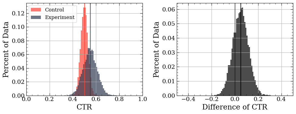
Simulated data showing the CTR for two groups of visitors (left) and the difference between their CTRs (right). Vertical lines indicate the mean.

Unfortunately, this approach has a big issue — it doesn’t account for user variation. The above distributions have a large range of values. The world is chaos random, and like it or not, we need to acknowledge it. In short, a measurement without an error bar is of little use.

Typically, one would handle these uncertainties using a “Frequentist” approach. Broadly speaking, with Frequentist testing, you create a null hypothesis (typically that there is no difference), observe data, and then calculate whether the data violates the hypothesis. This is usually done by working with a Frequentist summary statistic of the data (i.e. some number that captures your data). As the graph below shows, you create a reference distribution based on the null hypothesis, determine what some critical threshold would be for your calculated statistic, and see if your data’s statistic surpasses that threshold.

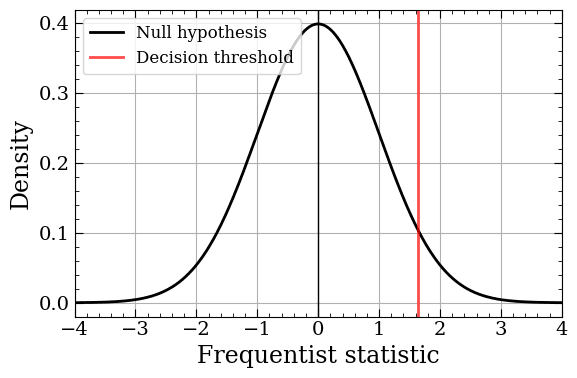
The distribution for the Frequentist statistic based on the null hypothesis. The vertical line indicates the threshold for decision-making. Data with a larger statistic than that are “significant”.

Contradicting yourself in order to achieve a result can cause confusion and lead to errors in communication. To briefly summarise a century of statistical debates, there are a few further pain points with Frequentist testing:

• Arbitrary decision criteria — The crux of “Does the data violate the hypothesis” is the infamous p-value, an arbitrary threshold. So arbitrary, in fact, that it’s from a book released 100 years ago by British mathematician Ronald Fisher¹. On page 45, he writes:

  (It is convenient to take) the value for which p = 0.05, or 1 in 20 … as a limit in judging whether a deviation is considered significant.

• What’s the plausible range of difference? — Often Auto Trader colleagues appreciate the world is chaos random. Thus, they’d like to see the most likely values for the CTR difference between the groups. There is partially a way to answer this in the Frequentist framework (e.g. confidence intervals), but their interpretation is nuanced and comes with limitations.

We wanted to find a solution to the above problems and better communicate with stakeholders. This motivated our exploration of the “Bayesian” framework.

The new approach

In the Bayesian framework, we are interested in creating a probability distribution for our metric. This probability distribution, the Posterior, allows us to answer many business questions. In our example, we can represent the probability of the CTR given the observed views and clicks as \(P(CTR\|Views, Clicks)\).

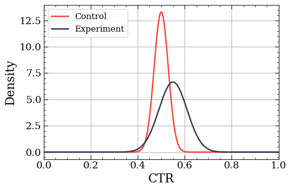
Posterior probability distributions for the two groups.

Note that the Posterior represents the uncertainty surrounding the metric, not just the ratio of clicks to views. This uncertainty comes from two sources: the Likelihood and the Prior. The Likelihood, \(P(Views, Clicks\|CTR)\), encapsulates the randomness of generating data. Essentially, how likely would a given CTR be if we had a given combination of views and clicks? The second source of uncertainty, the Prior, \(P(CTR)\), represents our initial belief about the value of the CTR. This is a subjective decision. Perhaps we have no idea, in which case we can make it an “uninformative” Prior and say all CTR values between 0 and 1 are equally likely. But we usually have a decent idea for metric values based on years of historical data. In practice, we recommend erring on the side of caution and using “weakly informative” Priors. If your Prior is causing an unwarranted bias in your Posterior, it’s likely too strong, or you don’t have enough data! Finally, there is the normalisation term, \(P(Views, Clicks)\), a nuisance term that merely ensures the resulting Posterior distribution is a valid probability distribution. It’s such a nuisance term that the Bayesian methodology wasn’t widely used for many years. Altogether, we get Bayes rule:

\[P(CTR\|Views, Clicks) = {P(Views, Clicks\|CTR) P(CTR) \over P(Views, Clicks)}\]

The above is a lot of words, so let’s visualise it. The plot below shows how our initial Prior changes as we add more observations to our dataset. Let’s (incorrectly) assume our CTR has a mean of 0.25, but we’re not certain, so we spread out the probability, creating a weakly informative Prior. Then we’ll simulate data and calculate the Posterior using Bayes rule. We’ll repeat this process, each time drawing more data. Since this is a simulation, we know the true mean (the dashed black line). We can see that as we draw more samples the Posterior quickly captures the true mean, despite the mis-specified Prior.

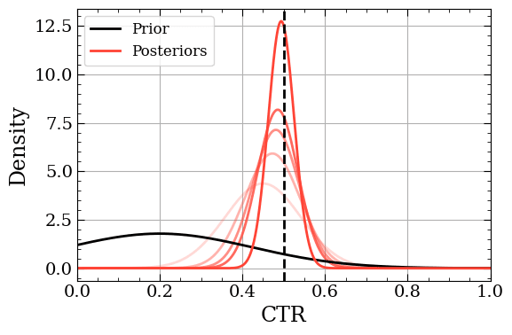
As more data is added (the shading becomes darker) the Posterior narrows in on the “true” value.

Knowing when to stop: Expected Loss

Let’s assume for now we’ve created our Posteriors by selecting an appropriate Likelihood and Prior for each group. These Posteriors reflect the range of values we expect for the CTR. The question now becomes, what do we do with them?

First, we can ask: Is the experimental CTR better than the control CTR? One way to answer this is via calculating the total probability that the experimental CTR is better than control’s CTR. This is called “Chance to Beat” and is surprisingly simple to calculate². We randomly sample from each Posterior, calculate the difference between the CTRs, and repeat the process many times (say 10,000). Doing that will yield a plot like the one below. This plot accomplishes three things! First, it showcases the most likely difference between the groups (the dotted line). Second, it visually demonstrates how certain we are of this difference (the range of values). Finally, calculating the fraction where the difference is > 0 (the highlighted area) will get your Chance to Beat metric.

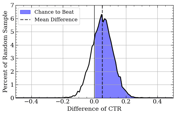
A histogram of random samples for the difference between two groups. We can estimate the mean difference, the range of plausible difference values, and the Chance to Beat all with one plot!

But wait, there’s more. The following concept, called “Expected Loss”, is based on a paper written by another statistician at VWO. The motivating idea for Expected Loss is that not all mistakes are equal. If we, by chance, pick the wrong variant, a 10% drop is much worse than a 0.2% drop.

To get the Expected Loss we first need to compute the Loss. Each randomly sampled difference between the Posteriors is multiplied by a reflected rectified linear unit (RReLU). Mathematically, this is simply: \(Loss(CTR_{Exp}, CTR_{Ctrl}) = Max(0, -1*(CTR_{Exp}-CTR_{Ctrl}))\). This function returns 0 if the experimental CTR is higher and the absolute value of the CTR difference otherwise. Calculating this Loss for all our random sample pairs and then getting the average gives us our Expected Loss.

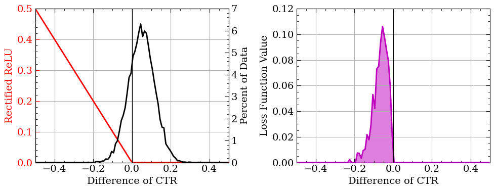
We can calculate the Expected Loss, which is sensitive to both the probability of the difference and how extreme the difference is.

The Expected Loss is in the same units as the metric. Thus, you can essentially read the value as a risk. In this simulation the Expected Loss is 0.04, meaning you’re risking, if you’re wrong, dropping from 0.50 to 0.46 CTR. Altogether, these values and distributions do a much better job of answering the questions our stakeholders are asking. Further, it places the emphasis on balancing risk and reward rather than a binary decision.

However, we must admit our criticism of thresholds in the Frequentist approach is a tad hypocritical. As it turns out, Expected Loss can itself be used as a threshold, should you desire, to terminate a live experiment. You merely wait until enough data has been collected that it falls below some pre-set value (typically around 1% of your control metric value).

The Expected Loss can drop below our chosen threshold due to one of two things:

• The Posteriors are sufficiently separated such that one of them has little to no weight on the negative side of the difference histogram.
• Enough data has been collected, and both Posteriors have shrunk sufficiently that the risk of making a mistake is small enough to not matter. This can occur when both variants are effectively identical.

The threshold can be adjusted depending on the risk tolerance for that particular metric at the cost of the experiment’s duration.

What it looks like in practice

We wrapped up the above methodology into a Python package, which is internally available to our colleagues in the Analytics Group via pip. Since the methodology was new, we wanted it to be as easy as possible to use while still being flexible enough to adapt to specific use cases.

To use the package, a few key decisions are required:

• Likelihood for the test metric — The underlying function that generates the observed data.
• Expected Loss Threshold — How much risk are they willing to take?
• Prior strength — A very weak prior is used as the default, but the analyst can choose to make it stronger if needed.

Choosing the correct Likelihood is the most important decision out of the above. The package comes with several special Likelihoods that contain conjugate Priors (a topic we discuss in the next post). Briefly, this special subset of Likelihood-Prior pairs covers many use cases and has favourable mathematical properties for creating Posteriors.

How long does it take?

As an added bonus, the package can perform a helpful pre-calculation. Before starting an experiment, it is important to know how long it will take, as a test that will take 3 years to gather enough observations to make a decision is pretty unhelpful! To aid those initial conversations, our package contains a time_to_result method. The worst-case scenario for this Bayesian framework is that both variants are identical. If this occurs, the only thing reducing the Expected Loss is reducing the variance of the Posterior (rather than reducing the overlap of the Posteriors).

We can use this fact to compute the expected time to run in the worst case. If we know the approximate value of the metric being tested and the typical number of events per day (which is almost always the case), we can empirically compute the time to run. We simply simulate data from identical experiments of increasing size, e.g. 10, 100, 1,000, 10,000 visitors, and observe how the Expected Loss decreases with experiment size. From there we can work out the time to observe that many events.

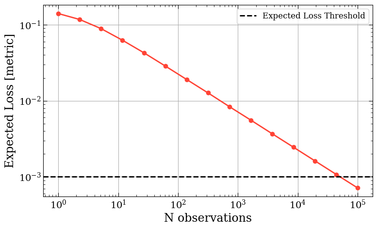
Expected Loss as a function of the number of observations in the case both variants are identical.

What did people think?

The above represents a significant shift in how we perform A/B tests at Auto Trader and ensuring the adoption went smoothly was critical. We have a forum for discussing current tests, raising concerns, etc. It was a great place to get ideas and feedback during the development of this methodology. Throughout our discussions, the main issue was selecting the likelihood. In an attempt to solve this challenge, we created a generalised approach, which we discuss in more detail here.

From a stakeholder perspective, we now speak a more familiar language, discussing risk and chance to beat rather than overly simplistic decision criteria. This more visual representation better aids us on the analysis side to help the stakeholder make a more informed decision on what to do next, which, in the end, is what an A/B is all about.

Summary

Overall, the move towards a Bayesian approach has been a very interesting one and a real shift in how we view experimentation. It addresses our frustrations with the Frequentist methodology and has meant that we can move faster with our experiments and have greater confidence in our decisions. It also makes the subjective choices in an experiment more explicit, such as the Expected Loss threshold and what we expect the data-generating process to look like.

In the companion post, we discuss some improvements we’ve made since the initial roll-out to make it even easier to use by effectively removing the need to choose a Likelihood-Prior combination.

_{[1] Fisher, R. A. (1925) Statistical Methods for Research Workers. ↩}

_{[2] We are quick to note that we are actually just estimating the “true” Chance to Beat. To compute the actual metric (and the other metrics discussed later), we’d have to solve some tricky integrals. Sometimes, the integrals don’t even have closed-form solutions! However, the estimation is quite robust if you sample enough from the Posteriors. ↩}

Share:

Enjoyed that? Read some other posts.