Here at Auto Trader we are always striving to improve the experience for both our buyers and sellers. In this blog we describe how we have used machine learning to estimate how attractive different adverts are to car buyers, in order to improve how we select which adverts to display in our search results. We elaborate on how we followed the Discovery -> Production process discussed previously to deliver the project, and the lessons we learnt along the way!

Introduction

When a buyer, looking to buy their next car, visits our website and searches for a vehicle, they are presented with a list of search results:

We want car buyers to click through into as many full-page-adverts (FPAs; the webpage displaying all the information about the vehicle for sale) as possible, for three reasons:

1. Good buyer experience– We want the buyer to find their ideal next vehicle quickly, but we want them to feel that they have made an informed choice by comparing what is available.
2. Good seller performance– We know that the more times an advert is viewed, the more likely that vehicle is to sell.
3. Good for Auto Trader– Happy buyers and happy sellers means a happy Auto Trader.

FPA views are also one of the Key Performance Indicators which we report to the market. We also directly make money from buyers clicking on our PPC (pay-per-click) slots. Improving the click-through-rate (CTR; the rate at which buyers click through from search results into FPAs) is a win, win, win situation.

We wanted to determine which adverts our buyers want to click on, i.e. which adverts are “attractive” to them. Coming up with a hardcoded list of factors that make an advert “attractive”, however, is hard to do. Things like our price indicators and the number of images could play a part, but so will things like image quality which is very hard to measure.

Instead, we can utilise the vast amount of data we collect from our website each day and use statistical methods to “learn” which adverts our buyers want to click on. We want to learn an “attractiveness” value for each advert, but to do this we need to take into account the other factors that affect whether a user clicks on an advert or not. This includes things such as the device type the buyer used to visit Auto Trader, which page of the search results the advert was displayed on, and how far down that page it appeared.

We can also try to capture how “relevant” the advert is to the buyer, by looking at how many search filters the buyer used, and how many search results were returned in total. Looking at the number of search filters a buyer has used can tell us a lot about the attractiveness of the adverts shown to them; for example if a buyer has set lots of filters and they still don’t click on any of the adverts shown to them, then this tells us that those adverts are probably quite unattractive to that buyer! Conversely, if the buyer hasn’t applied any of the available search filters, then we can probably surmise that any adverts they do click on are very attractive to them.

Prototype

Data exploration and prototyping is undertaken using Databricks and Apache Spark. These tools allow us to handle the huge volumes of data generated by our buyers’ interactions with our website and quickly build up a process to clean, transform and model the data. The prototype machine learning pipeline for this project consists of three stages, with each stage written in a separate Databricks Python notebook (Databricks supports Scala, Python or R; our Data Scientists tend to prefer Python for prototying and exploration). A machine learning pipeline is a set of connected steps that are needed to execute the full process and produce results.

1. The first stage in our pipeline collects a week’s worth of data on which adverts were displayed on Auto Trader’s search pages and any onward clicks to their FPAs;
2. The second stage of the pipeline then cleans the data and ensures that each advert in our training dataset has had sufficient search impressions in the last week. The more impressions an advert has, the more accurate the advert attractiveness estimation will be;
3. The third stage then fits a logistic regression model to the data using Spark ML, including features such as the device type, search page, advert position, search filters; and an advert_id feature. On average we are fitting this model to around 175 million rows of data each day, with around 375,000 levels in the advert_id feature. We explicitly do not fit an intercept, as we want a coefficient for every level in the advert_id feature. Fitting this model allows us to give each advert an “attractiveness score”.

It seems the Spark ML libraries are generally written with prediction in mind, however, in our case we are not trying to make predictions of click-through-rate. We want to extract the coefficient for each level of the advert_id feature, as this represents the “part” of the advert click-through-rate which is due to that specific advert. Taking the exponential of the coefficient for an advert_id gives us the “attractiveness score” for that advert. We can also use the estimated probabilities of click and no-click for each row of data to estimate the standard error of the attractiveness scores, using standard statistical methods.

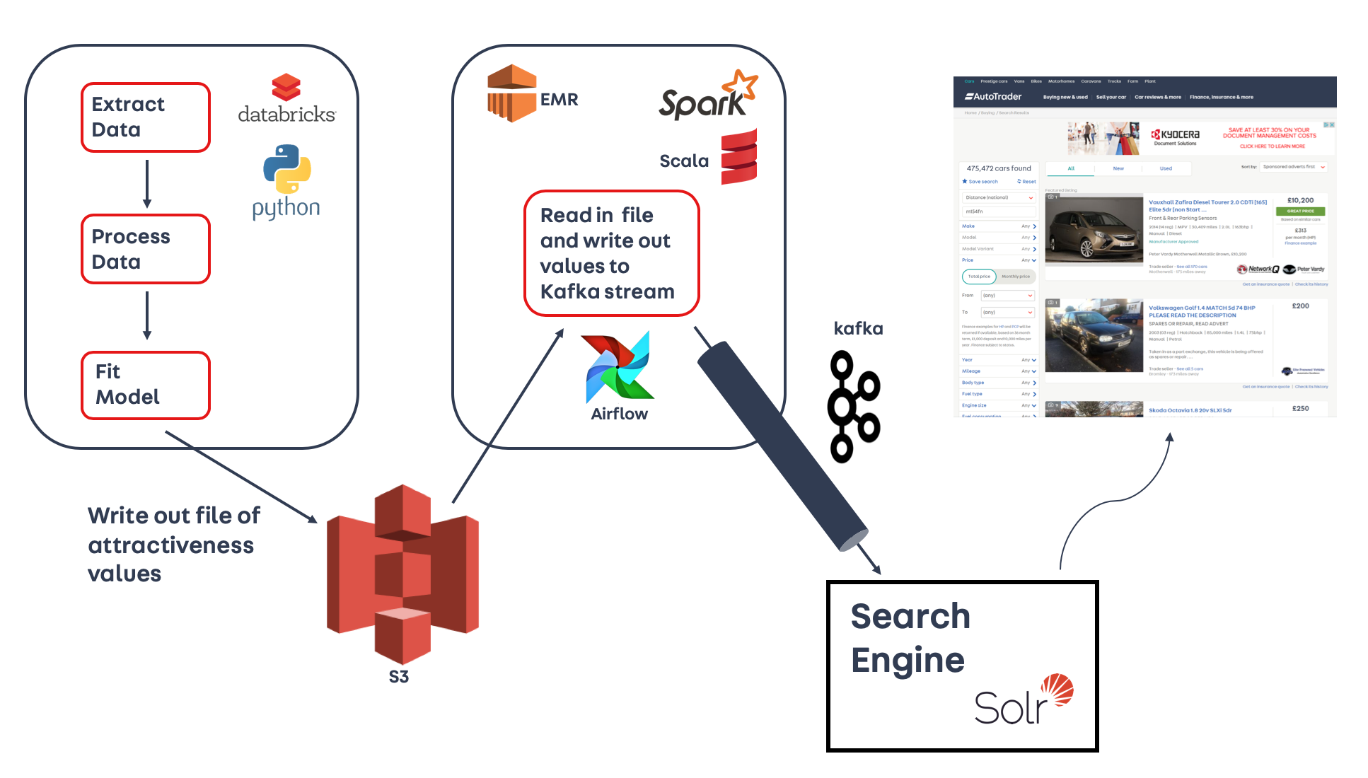
We wanted to test that using attractiveness as a weight when selecting which adverts to display would provide us with an increase in CTR. To do this before investing the time and effort to productionise the pipeline, we utilised the scheduling tools in Databricks to run the three notebooks in the pipeline each morning. The results were then written out to our data lake in Amazon S3 (to learn more about what a data lake is and how it fits into Auto Trader’s Data Platform, check out this video ). We had to write a separate spark job to then read in the results each day and emit them to a Kafka stream, which our search engine could pick up. The diagram below shows a schematic of the prototype pipeline.

We ran 5% and 50% tests in our Promoted Listing slot (a paid-for slot in our search listings which is designed to give adverts more prominence) and saw a large increase in CTR, which was very promising! This convinced us that it was worth the effort to productionise the product.

Productionisation

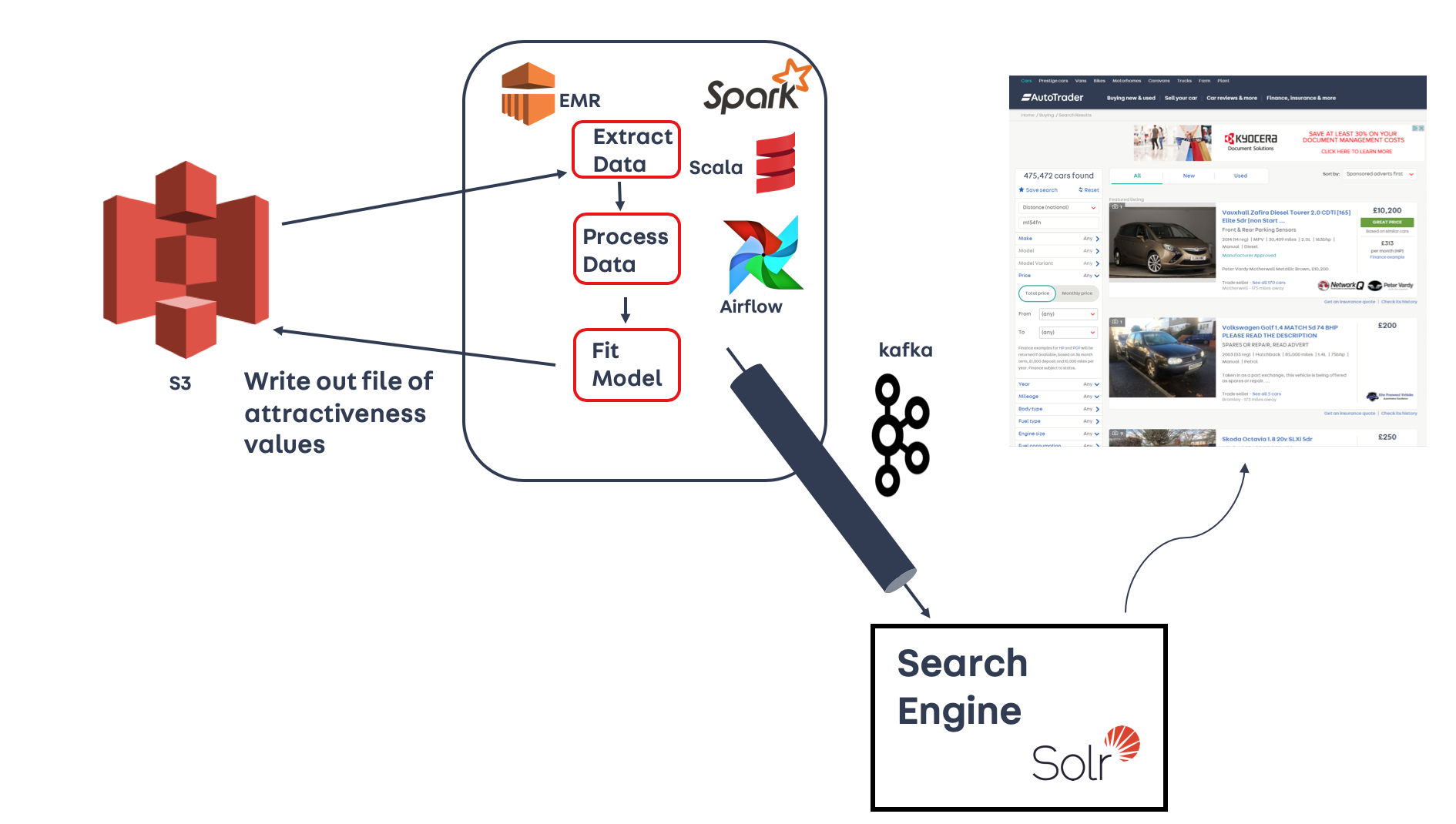
The first task we had to approach was to port the three Python notebooks into Spark jobs written in Scala (all of our ETL jobs are written in Scala). As we had moved away from the Databricks ecosystem, we also had to find an alternative way to trigger those Spark jobs. We used Apache Airflow to schedule the Spark jobs at the required time and in the correct order. The diagram below shows a schematic of the production environment (a lot tidier than the prototype!)

Migrating from Databricks to our production environment was not as easy as we originally thought. In the next two sections we are going to cover what the execution looked like, and some of the key things we learnt during the productionisation process.

Execution

We were faced with three main tasks:

• Convert all three Python notebooks into Spark ETL jobs written in Scala;
• Port from Databricks (scheduling and compute) to using Airflow and EMR in our production ETL environment;
• Produce exactly the same output as the prototype. Nothing less, definitely nothing more.

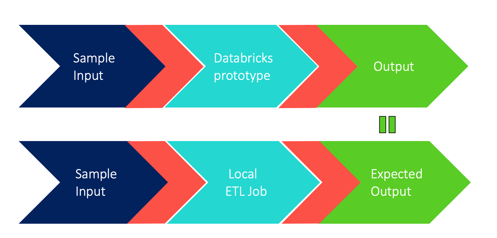
It was pretty clear that we had to follow a methodical approach to tackle these tasks. In order to replicate the output of the prototype, we used a sample data set to generate a reference output. This was then used by the production integration tests to confirm the performance of our Scala ETL jobs.

Once we finished the implementation and all integration/unit tests were passing locally, we moved on to deploying our ETL job to the cluster where it could access the full-scale datasets.

The ultimate test was then to check whether we had produced the same output as the prototype… which we didn’t – for quite a long time.

Gotchas and Learnings

Eventually, we got there, but it was definitely a bumpy road with lots of gotchas and learnings. We will list some of the most interesting ones below.

Know your data

Close and frequent collaboration between data scientists and software engineers was essential and played a key role in delivering this work. Understanding how the data was initially shaped, and its ongoing transformation throughout the process, was critical during implementation and debugging.

Checkpoints and feedback loop

One of the most frustrating moments we had was around how much time it would take for a process to finish and finally be assessed for correctness. This is due to the fact that the input data in the production environment is huge (typically 175 million rows) and would take on average 3 hours to complete all tasks. To put it into perspective, this is about a third of a working day which meant that the feedback loop was quite slow and painful, but this is expected when processing that amount of data.

We would then use Databricks to trace back which piece of input data was causing the inequality, and finally include it in our local version of the ETL job to replicate the bug locally. This meant that the feedback loop through integration tests was almost instantaneous and any future related issues would be flagged up by the integration test before we would push them up in the production cluster.

Evaluation strategy and monitoring

One of the main outcomes of productionising this work is increased confidence.

• confidence in whether it works or not,
• confidence in any further changes,
• and if something is broken, confidence in figuring out which part of the process is broken.

We also wanted to have confidence that the output is correct, so we added soft integrity checks to automatically evaluate the data at each stage of the process.

Pre-production

Each Databricks notebook had a dependency on the previous notebook, and on the input-datasets being available in S3. Sometimes the whole pipeline would fail to run due to one of the datasets being unavailable or delayed in its production.

Each morning the data scientist had to manually log-in and check that the notebooks had run successfully, and re-run them if not. Key data and model evaluation metrics were calculated at the end of the final notebook, and again these needed to be checked manually by eye every day, to be confident that the results being produced were OK.

This was a very manual and time-consuming process and included having to log-in and check the notebooks on weekends. Even when the data scientist was on holidays, we had no one to have a look at the advert attractiveness results and resolve any issues due to the high complexity of the problem and the required expertise.

Post-production

Everything is a lot easier! Now that everything is scheduled within Airflow’s ecosystem, the ETL jobs will only run on the scheduled time if the dependent datasets are available or when they become available.

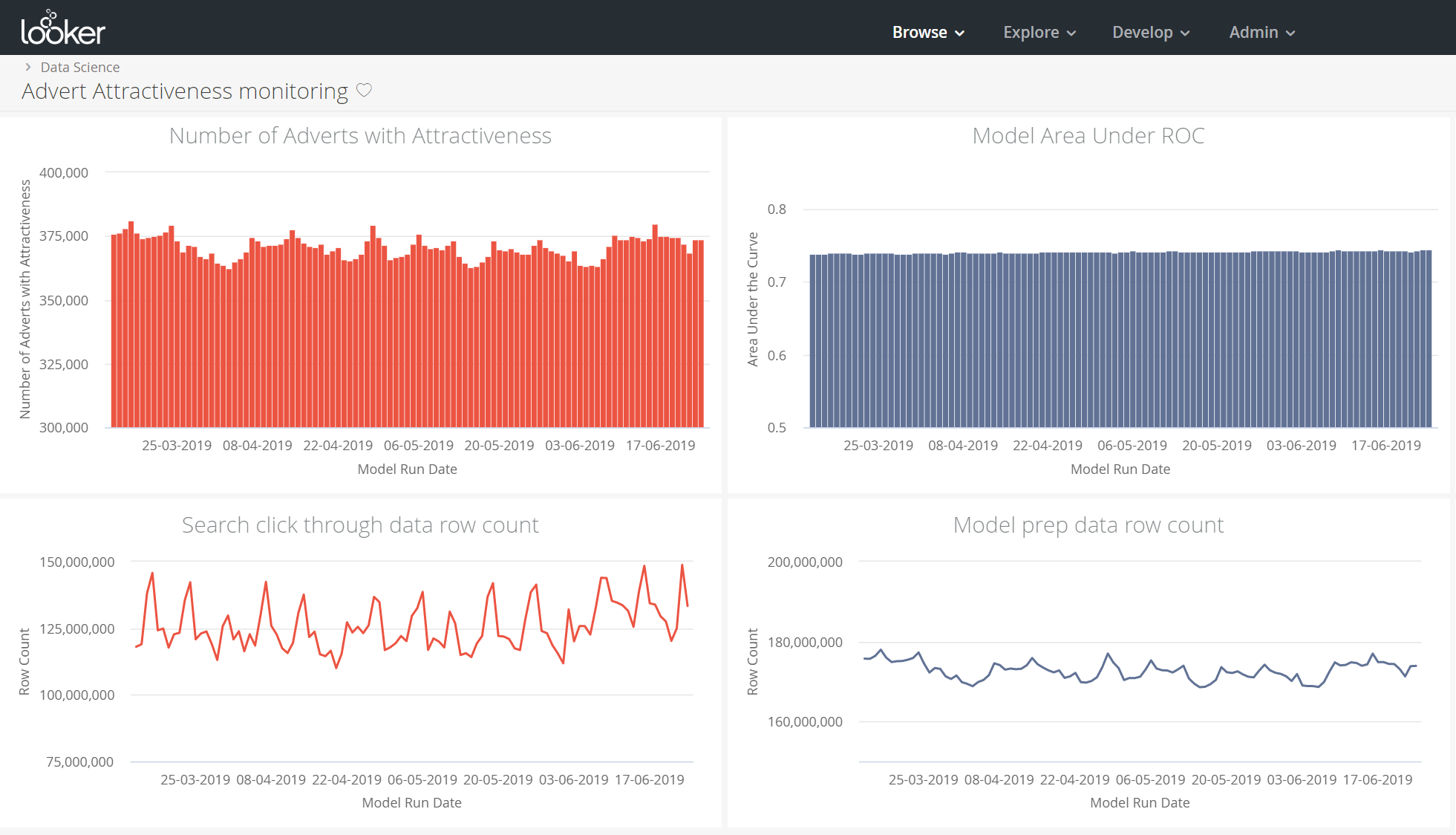
Each key evaluation metric is also now available in a Looker dashboard (a section of which is shown below), which can be monitored.

Each dataset generated by the spark ETL jobs is automatically run against integrity checks to detect any abnormality in terms of row counts, and if one of the integrity checks fails a notification is automatically sent to the appropriate team.

Summary

In summary, we learnt a lot during this project! It was a genuine collaborative effort between data scientists and software engineers, and we all gained a huge amount of experience using the different parts of our Data Platform toolkit. We are now exploring how best to utilise the advert attractiveness scores to improve the car buyer experience on our website and apps. Watch this space!

Share:

Enjoyed that? Read some other posts.