At Auto Trader, we have multiple machine learning models to predict and score properties of the advertised vehicles on our platform, from valuations to desirability. With circa 8,000 new adverts listed each day, how do we generate scores for all the new adverts that have limited observations? How do we ensure that these are fair estimates of their long-term value, and aren’t going to erratically vary day to day? In this post, we’ll cover how we have addressed these problems in the case of one of our core models, Advert Attractiveness, which scores adverts based on their quality.

Intro To Advert Attractiveness

The core of our business at Auto Trader is helping people to find their next vehicle (be it car/van/truck/caravan etc.!) as easily as possible. As such, a question we need to be able to answer is “which adverts are the most attractive to our users?” Several years ago we created Advert Attractiveness specifically for that purpose (we have a blog post about it). At its heart, the Advert Attractiveness model looks at the response of users towards a given advert, while accounting for the context it has appeared in (e.g. desktop vs mobile, position of the advert on the page), and the user’s behaviour as well. The aim of this is to minimise the role that luck plays in an advert’s response in order to find the best quality adverts.

The original model only scored a subset of the advertised cars on our site. This was because it needed a reasonable number of users to see each advert (we’ll refer to these as observations) to produce a reliable score. This was done with a set of hard thresholds on the number of observations each advert had to acquire before getting a score, which meant we had limited coverage of circa 80% of car adverts scored. As we also wanted the score to be relevant to the current state of the advert we have a fixed observation window of seven days. This is because imagery, pricing etc. can all change over time, and we don’t want to saddle a newly improved advert with a low score because of its low response from weeks ago. The flip-side of this is that some adverts will never get enough response to be scored, particularly in our non-car channels.

Since its initial release we have continuously been working on the Advert Attractiveness model to address the above constraints; this has proven to be a challenging and very satisfying endeavour.

Extraordinary Claims Scores Require Extraordinary Evidence

What Advert Attractiveness does is compare the observed response to what we would have expected given the set of contexts that it has appeared in. The original model simply took the raw response as the input to that comparison, leading to several problems due to the ratio being erratic early on when there is little data. This is why the original model also imposed a minimum number of observations before scoring, but ideally we’d be able to score all adverts the moment they are live on the site. We needed to find a solution to balance the want to score as soon as possible and the fact that the fewer observations we have the less sure we are about the advert’s quality.

Fortunately, as we have ~500k adverts on Auto Trader at any one time, we have a good idea about the distribution of the response levels of our adverts. For example, in any kind of metric which is based on click-through rate the distribution approximately follows a Beta distribution. If we know nothing about an advert we can still have an idea of what its likely click-through rate will be based on our prior knowledge of the distribution of all adverts on the site.

Those familiar with the Bayesian view of the world can probably see where this is going. We have a prior distribution, informed by the performance of many previous adverts, which we can update as more and more information comes in. Eventually, with enough response, our initial prior assumptions no longer practically impact our posterior¹ estimate of the response. This process of updating with additional information is illustrated below.

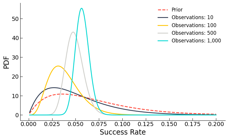
The y-axis shows the Probability Density Function (PDF), which means that the area under each curve represents a probability and each curve has unit area (we know the result will definitely lie between 0 and 1). You can see that we start off with a broad prior (red dashed line), which narrows as we gather more information about the advert.

The power of this approach is that we no longer need any hard (and arbitrary) cut-offs for when to score an advert. Instead, we start off with a reasonable estimate, based on the general population of adverts we have on the site, which we continually refine with additional evidence (as illustrated in the plot above). This approach allows us to score practically any advert fairly, not only for car adverts, but vans, bikes, caravans, motorhomes, and our industrial equipment (known as Truck Plant Farm).

In addition, we benefit from a negative feedback loop. If an advert scores poorly, then it will be shown less in some of the positions we are interested in (such as our Promoted slot). However, this means that we have fewer observations, which tends it back towards the mean. Similar for high-scoring adverts, as we show those more we get more observations, increasing our confidence in the estimate, making it hard for an advert to maintain a high score by luck alone. This negative feedback loop is far more desirable than a positive cycle, where adverts will accelerate towards the extremes.

With our raw observed response now restrained in the case of low data, we have a much more reliable and stable model, which still allows great adverts to shine. However, this fix exposed a similar yet more subtle problem.

Fishy Results

In the previous section, we talked about how we have a fair estimate of an advert’s response, accounting for the noise inherent in having limited observations. However, there is a second factor that we have yet to consider. When comparing the ratio of true (or our best estimate of it) and expected response we have only altered the former, not the latter. As it turns out this can still lead to extreme scores at very low numbers of observations. This is easily seen in a plot we lovingly refer to as “the fish”.

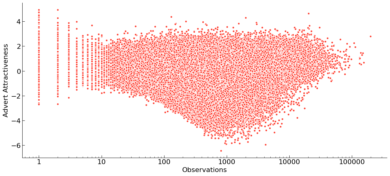
What we can see here is the Advert Attractiveness score against the number of observations we have of each advert. Note the x-axis is on a log scale. The shape of this plot arises from two main mechanisms, the first being the impact of our aforementioned prior - it is difficult for adverts to get extreme scores with low numbers of observations, and so we see the body of the plot widen as observations increase. However, we also use Advert Attractiveness to inform which adverts we show to users on our site in slots such as our ‘Promoted’ position. This means that as we become more confident in an advert’s poor score we are less likely to show it, thus making it difficult for low-scoring adverts to get a very high number of observations causing the second half of the plot to narrow, leaving just the high-scoring adverts with very high numbers of observations.

There is a third feature of the fish plot: the “tail”. This is what we are concerned about, as the scores here become erratic. The root cause of the problem is that while we have a prior on our observed response, the ratio to the expected response can still be unstable as the denominator can vary substantially. The expected response can vary significantly because of the context an advert can appear in. Imagine that an advert’s first observation is at the top of the page for a very engaged user, even in this scenario it is perfectly likely that the advert won’t be interacted with. If we compare with the case that advert had appeared right at the bottom of the page, the value of the observed response is the same (no response), yet the expected response is very different. We need to somehow capture the fact that even though the expected response maybe higher, we won’t be able to measure any difference until we have several observations.

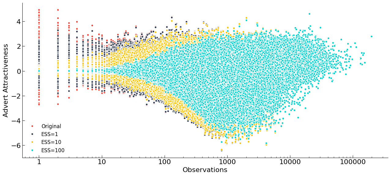
We looked into multiple ways to apply a similar methodology to the denominator as for the numerator, however we often saw strange artefacts, such as an empty arc in the “fish”. Our solution was to apply an effective sample weight to the Advert Attractiveness itself. Fortunately, we can approximate the distribution of Advert Attractiveness scores as a Gaussian, and so we can apply an adjustment to the raw score, s_r, as

\[s = \frac{1}{n_e+n}(\mu_0n_e+s_rn)\]

where n is the number of observations, n_e is an effective sample size (it arises as a ratio of variances, but we won’t go into detail here) and μ₀ is the mean of our prior. You can sense check the above equation by looking at its behaviour when n (the number of real observations) becomes large, the score (s) tends to the raw estimate, s_r. Below we have some examples of different effective sample sizes, including some extreme values that nicely illustrate the effect of this change. For our purposes, we just want a value that reduces the extreme values, somewhere between 1<n_e<20.

Summary

Since its first release into the wild, we have continuously monitored Advert Attractiveness to see where we could improve it, and in this blog post we have discussed just a couple of changes we have made to it (there have been many more!). In order to allow us to score almost all adverts on site we have introduced prior weightings. This meant that even adverts with few observations could be given a score that was fair, smoothly changing with increasing data. The introduction of the prior on the observed response was a success, however, it exposed the issue with the expected response term being unstable at very low numbers of observations, requiring an additional prior.

The addition of these priors has been the key to allowing us to maximise coverage across all our different vehicle categories at Auto Trader. Consequently, we have improved not just the user experience with these more reliable scores, but also the machine learning models that use Advert Attractiveness as an input feature.

_{[1] For the purposes of this post you just need to know that the prior distribution is our initial assumption about the system and the posterior is the new best estimate after combining the prior with new data.↩}

Share:

Enjoyed that? Read some other posts.