How similar is a Ford Focus to a VW Golf? Is a Focus more like a VW Polo…?

At Auto Trader the question of how similar two vehicles are to each other occurs frequently, whether it be in the context of recommendations, helping retailers understand who their competitors are, price valuations etc. In this post we will describe one of the ways we have to compare apples and oranges (or in this case coupes and hatchbacks!).

Fundamentally, car buyers are the ones who decide if two vehicles are similar or not; if two vehicles are frequently looked at together by the same users they must be somewhat similar. The method discussed in this post comes from the field of Natural Language Processing and is an interesting example of how, with a bit of lateral thinking, powerful insights can be gained from applying techniques from seemingly unrelated areas.

Why not use use buckets?

Perhaps the simplest way to answer “Are these vehicles similar?” is to group together vehicles into ‘buckets’ that are physically related somehow. E.g. All petrol cars in one bucket, electric in another etc.

Once the buckets are decided then you can easily say that all vehicles in the same bucket are ‘similar’. Even this kind of simple approach is valuable as it is easy for anyone to interpret, and depending on the question might be all that is needed, such as “Are Electric cars selling faster compared to a year ago?”.

While bucketing might be easy to interpret and implement, choosing the splitting criteria is often difficult and highly subjective. If we are trying to recommend new vehicles to a user on our site, and they have just looked at a Ford, we could try recommending to them any other Ford, and likely see little success, as our bucket is far too broad; a Transit is very different to a Fiesta. We could narrow the bucket to model level, or bucket based on body type (Hatchback, SUV, etc…). We could go all the way down to what we call at Auto Trader the derivative level. A derivative is a unique combination of make, model, trim, fuel type and several other properties. On Auto Trader there are approximately 45,000 different derivatives advertised at any one time, compared to ~1,300 unique car models. In contrast to bucketing by make, bucketing by derivative is far too narrow for most applications, such as recommendations.

A problem we have with bucketing is its all or nothing approach, a vehicle is either in a bucket or not. If we bucket by model, then we are implicitly assuming that a Ford Fiesta is nothing like a Ford Focus, or a VW Golf. Intuitively we know this is not true, and so we need a way to quantify how similar different buckets of vehicles are to each other.

Co-occurrence

One way to measure how similar different groups of vehicles are to each other is to create a co-occurrence matrix, which shows what fraction of the time two groups are viewed together by the same user. Below we have co-occurrence matrix at the make-model level generated using data from Auto Trader, with ~45,000 elements, and models listed in alphabetical order. The brighter the colour the more likely the models appear together. You can clearly see the yellow line down the diagonal, as the probability that model A will be in the same session as one containing model A is exactly 1.

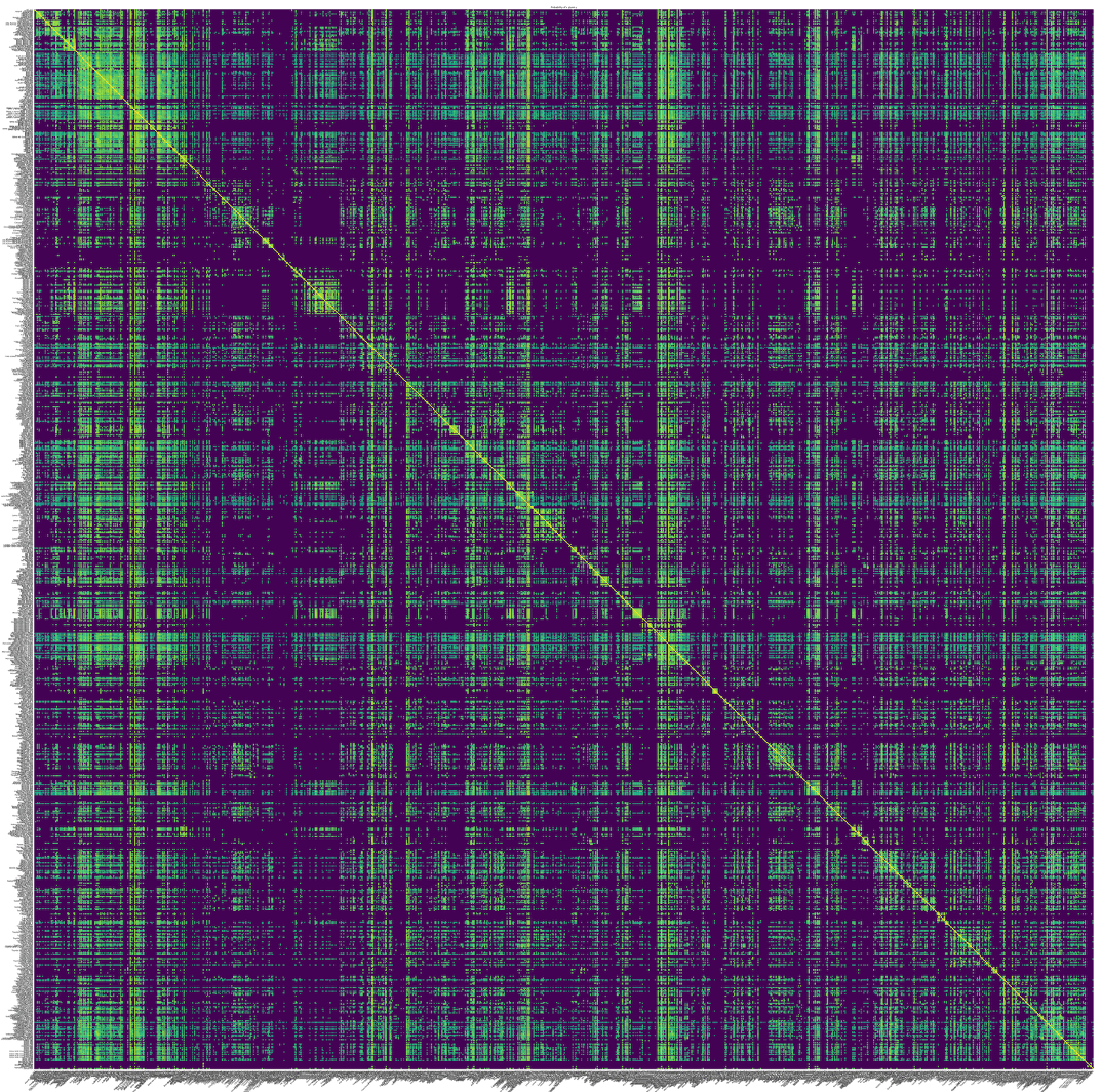
From this matrix, we have the probability that make model A will be viewed by the same user as make model B, or more precisely, P(A|B), read as the probability of A occurring, given B has been viewed. As the rows and columns are ordered alphabetically you can see see clear bright patches dotted around the diagonal line. In particular you can see a large bright patch in the top left corner, caused by all the Audis and BMWs. There are also many dark purple regions, these are where we have very few, if any, observations of users looking at both models in a session.

On the face of it this matrix could seem like an ideal solution for measuring how similar different buckets of vehicles are to each other, however there are several problems…

1. The matrix is huge, there are ~1,300 unique car models on Auto Trader at any one time, or 45,000 unique car derivatives. The number of entries in the matrix grows as O(N²), which means 1.7 million probabilities at the model level, and 2 billion comparisons for derivatives! If we wanted to compare every vehicle on the site that would be ~500,000² = 250 BILLION entries.

2. Related to above, the matrix is sparse, if not enough A/B pairs have occurred we get a poor estimate of the true probability, P(A|B), or simply no data at all (which is the case for most of the dark purple regions in the above plot). Some models are also rarer than others, we can pick out rare models by looking for columns in the above plot that are mostly dark. We might have enough data to say that a rare model A is similar to model B, but not enough for model C. If we knew that B and C are very similar, it would be nice to be able to infer that A is probably similar to C as well.

3. The matrix is only good for comparing pairs of vehicles, but users look at many when browsing, so what we really want is P(A|B,C,D,E…). Computing P(A|B,C,D,E…) directly for every combination of A, B, C,… quickly leads to astronomically large matrices, with the vast majority of terms 0, due to lack of data. To illustrate why this is, every additional term makes the array of comparisons grow by 1, e.g. P(A|B)→ O(N^²), P(A|B,C)→ O(N³). Even our basic make-model level matrix would grow to 2.2 trillion terms for just P(A|B,C)!¹

From the above we can see that the probability approach has its limits. Any calculation involving more than one condition (e.g. P(A|B,C)) quickly falls victim to sparsity issues, and even if we had limitless data, the computational expense to store and sort through all these trillions of terms is prohibitive. Clearly we need to find a better solution…

_{[1] Alternatively one could approximate with P(A|B,C,D,E…) ~ P(A|B)P(A|C)P(A|D)P(A|E)… but that assumes each event is independent, which is absolutely not the case here, leading to nonsensical results.↩}

Vehc2Vec: A possible solution?

Our solution to the above problems was to use vector embeddings, taking advantage of a technique in Natural Language Processing (NLP) called Word2Vec, but instead of using words, we are looking at vehicles, so imaginatively we have called our implementation Vehc2Vec. As you will see it has a lot of advantages over the previous co-occurrence method.

Word2Vec is an algorithm that takes a set of sentences, such as

[
[The, hungry, dog, ate, some, food]
[Shops, sell, food, and, other, goods]
]

and then builds a simple single layer neural network that predicts the words that are likely to appear close to the input word (a.k.a. the context).² The below diagram illustrates the type of network used, except in our case we look at car models viewed by a user in a session, rather than words in a sentence. (Source)

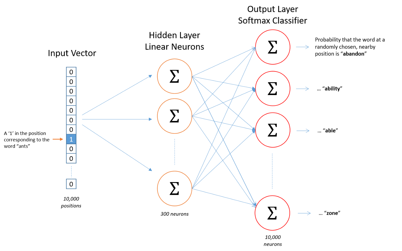
We will not delve deeply into how neural networks work in this post, but we will briefly describe what the above network aims to achieve. The input vector is N values long, where N is the number of unique words (or models/derivatives) in our dataset. One element in the vector is has the value one, the rest are zero. For example, the vector [1,0,0,…,0] could correspond to ‘a’, [0,1,0,…,0] ‘aardvark’ and [0,0,0,…,1] ‘zygote’. There is then a hidden layer, which in the diagram has 300 ‘neurons’. Each neuron is a weighted sum of all the elements in the input vector (hence the greek letter sigma, often used to denote a summing action). The output layer is similar again, another weighted sum, but this time the sum is constrained to be between 0 and 1, as we are wanting the probability that any given word will appear nearby to the input word. Constraining the output to be a probability is done with what is called a Softmax Layer (again we are skipping over the details). How to perform all these weighted sums is what the network learns over time. It takes an input, a single word, and then learns to output the probability for each of the N words that they will appear nearby to the input word.

The key idea in Word2Vec is that the hidden layer, which in the diagram is merely hundreds of elements long, rather than tens of thousands, encodes the meaning of each word. For example, the values in the hidden layer for “Apple” are likely similar to “Orange”, as both are common fruits, compared to say “Telescope”. Effectively what we have is a vector that represents each word in the dataset, and vectors that are ‘close’ together will appear in similar contexts, or be in some way interchangeable.

We measure the “closeness” of the vectors by computing the cosine similarity between any two word vectors, u and v, which is given by

If you are unfamiliar with the above term, all you need to know is that generates a value between -1 and 1. A value close to 1 means that the two vectors are almost parallel, while 0 means they are orthogonal, i.e. completely unrelated. Negative values are much more rare, and indicate a kind of ‘anti-similarity’.

We stress here that the actual values in the word vectors themselves (which is just the value of the 300 neurons in the hidden layer for a given input) are completely uninterpretable to a human. Think of it as a very strong form of compression, taking a vector that is many thousands of elements, and compressing it down to something much smaller. As you’ll see later, you can plot the vectors, and see interesting structure, but the each element of the vector does not have any interpretable meaning. Only when comparing word vectors, such computing the cosine similarity, do we pull out interpretable information.³

You might be starting to see how this can be used in the context of interchangeable stock. Our web traffic data can represented as sessions, containing car advert views (we’ll ignore other types of page view for now…) which look like

[
[Ford_Focus, VW_Golf, Ford_Fiesta, Vauxhall_Corsa]
[Porsche_911, Ferrari_358, TVR_Sagaris, Porsche_911, Porsche_911]
]

In our context, sessions are sentences, and car advert views words. From there it is a simple matter of training the network and we have a set of vectors for each make, model or derivative etc. But how do we know that the model is outputting sensible results?

_{[2] This is the skip-gram variant, there is also the Continuous Bag Of Words, CBOW, which takes the context, and predicts the target word↩
[3] Just because the vectors don’t make sense to a human, doesn’t mean they cannot be extremely powerful inputs for other machine learning models ↩}

Is it working?

So we now have some vectors, do they make sense?

The problem with unsupervised ML models such as Word2Vec is that there is no accuracy score or similar way to quantify how good a job it is doing, if we knew which vehicles where similar we wouldn’t need these abstract vectors in the first place! There are also many pre-processing steps and properties of the neural network we can tune, such as changing the length of the hidden layer and how many days of data we train on. How do we know we’ve tuned the model well? The easiest thing to do would be to output lists of “most similar vehicles to x” and manually check to see if it makes sense, but this is not quantifiable.

In order to choose the neural network properties we focussed on how stable the models outputs were. The logic behind this is straightforward, if we train the same model on two independent sets of data and get radically different similarity scores then the model is not very good, a Porsche should not be near identical to a van one day, and not the next! Consumer habits/wants do change over time, but over the course of two weeks the wants of buyers should have changed very little indeed. For two different weeks we compared the cosine similarity score for every pair of vehicles and plotted them, as below, in a 2D histogram. The left plot shows initial distribution of scores, whereas the right shows the same input data, but after tuning the pre-processing/training of the model. Ideally everything would lay along the diagonal 1:1 white line. As you can see there is a big difference between the two, we have even had to change the colour scales, so that the left plot wasn’t a faint red smear! Hopefully this shows just how important pre-processing is for getting the best results out of a model.

Now that we have seen that our model is stable, we need to examine its outputs. After all a model that always outputs nothing but zeros would be stable, but not very useful…

What does it look like?

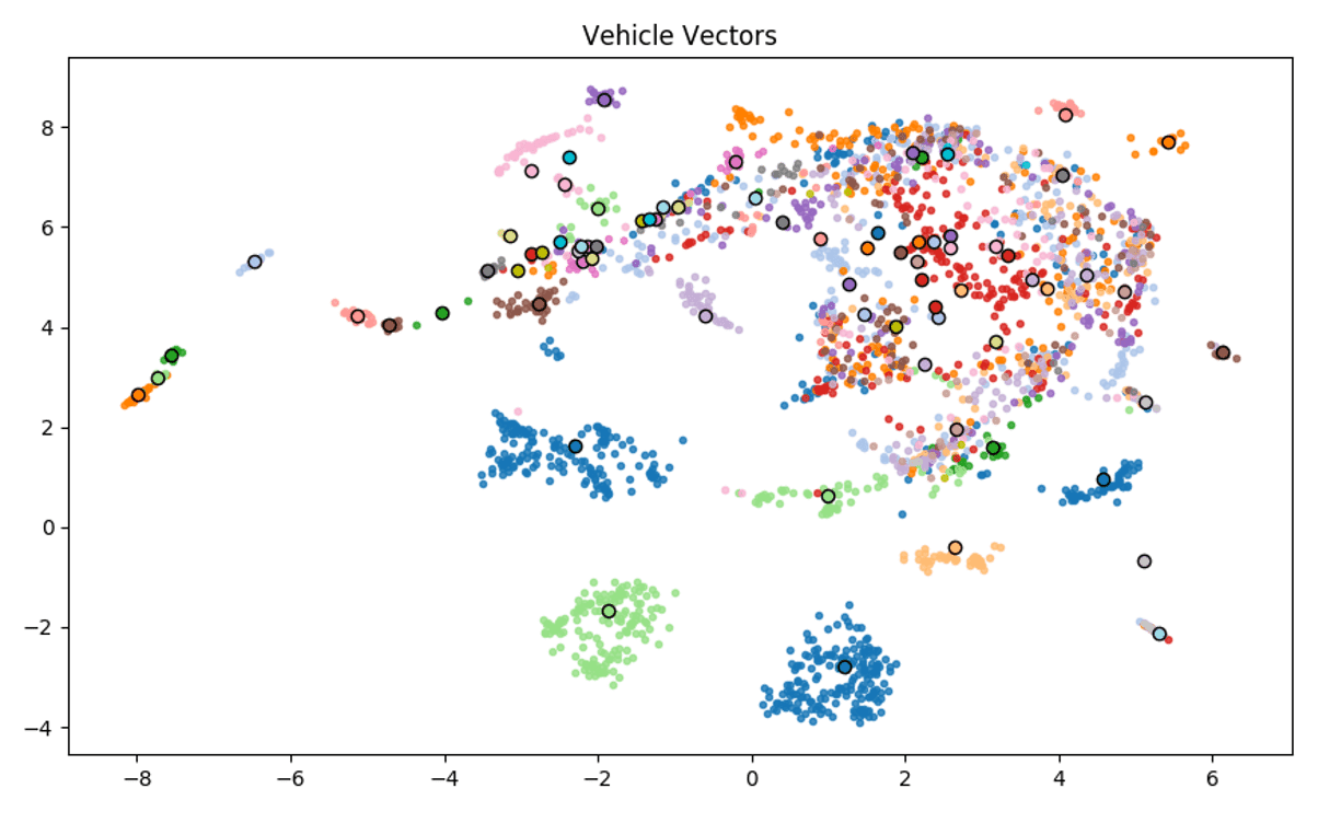
We are now happy that our Word2Vec (or Vehc2Vec…) model is stable. But what do the vectors actually look like? Visualising hundreds of dimensions at once is pretty hard, so instead we used a technique known as Uniform Manifold Approximation and Projection (UMAP) (read the Python package docs here), which allows us to project high dimensional data down onto a 2D plane, and is a popular tool among the Data Scientists at Auto Trader (comparing the differences between PCA, t-SNE and UMAP would be a whole other post in itself).

The below plot shows the projections of different vehicle generations, of which there are approximately 2,500 for cars. Each point is coloured by manufacturer, and for ease we show the mean manufacturer vector as a black edge point. Even from this plot we can see a lot of interesting information. The three clusters of points (2 blue, 1 green) towards the bottom of the plot are Audi, Mercedes and BMW, who appear to show strong self similarity. The messy area in the top right is comprised mostly of hatchbacks, where brand loyalty seems to decrease. The points to the far left (<-6) are supercar brands.

There are a lot of details we could go into here, looking at make level to derivative level vectors, colouring by body-type etc. Suffice to say that these vectors provide some very interesting qualitative insights. The fact that the insights also make sense is also gives us some more reassurance that the model is working well, and that we are ready to start applying it.

Applications

At the start of this post one of the motivations mentioned was better recommendations, and how the co-occurrence method struggles to deal with computing P(A|B,C,D…). We shall now discuss how these vehicle vectors can be used to generate recommendations.

If we have a user who has looked at 4 different adverts, we can simply average together each of the vehicle vectors to create a “user vector”. Note that there is a lot of literature out there on how to best to average word vectors together, the benefits of which we will not get into here. We can then compute the cosine similarity of the user vector and every vehicle vector, and come up with a ranking of which vehicles are most similar, and hopefully the most likely to view next.

We tested this by generating many user vectors from the first four advert views made, and then attempted to predict the 5th. We did not allow any of the previous 4 vehicles to be selected, as that is not so much a recommendation as it is a reminder, 20% of the time users looked at one of the previous 4 derivatives. 18% of the time the user viewed one of the top 10 derivatives (the top guess was correct 4% of the time). Considering the max accuracy was limited by aforementioned 20% cap, and that there are ~45,000 possible picks, this is a pretty good result! It also significantly outperformed our simple case model which simply predicted the most popular derivative of the same make and model as those viewed, which needed 11 guesses to achieve the same hit rate as the Vehc2Vec model with 1 guess.

“But” I hear you cry, “the model was trained on what users view together, isn’t this a bit circular?”. Yes that is true to an extent, and we have tested the model in other ways that are not based on user behaviour at all, such as predicting the which vehicles a retailer is likely to be selling and we have had similarly positive results. We are also using the vectors as inputs for some of our other machine learning models, where we need a mathematical representation of the vehicle advertised, which is proving to be quite powerful.

Summary

In conclusion, by applying the Word2Vec technique from the area of NLP, we now have a relatively lightweight, flexible methodology for comparing how similar things are to each other. And it can be applied to more than just vehicles, the exact same method can be used to compare retailers, or even user journeys.

Importantly, the ones who now determine which vehicles are similar are the users of autotrader.co.uk, rather than arbitrary criteria based on a vehicle’s taxonomy.

Finding the right method of tests to verify that the outputs were sensible was the most difficult task, but as we showed, extremely worthwhile, as it allowed us to tune the training process, giving far more stable results.

The “interchangeable stock” dataset is now commonly used by the Data Scientists at Auto Trader as a handy tool that can be input as features into other ML models that require an understanding of “how similar are these vehicles”.

Share:

Enjoyed that? Read some other posts.